Companion technical report · Simulated evidence · October 21, 2026
Short-Form Selection and Scoring: Companion Simulation Report
By Nedim Yel, Ph.D. Read the main methodological whitepaper for the formulation and practical findings. This report collects the implementations, study designs, diagnostics, detailed results and reproducibility files. All responses are simulated; no clinical instrument is validated here.
4. Assembly Solver Examples in R and Python
These assembly-only examples take a finite, nonnegative information matrix (grid points × items), content bounds, reading grades, reviewed enemy pairs and DIF exclusions. They do not calibrate a GRM, calculate Q₃, perform DIF testing or generate a crosswalk. Run these steps separately after checking dimensionality, fit, item permissions and calibration adequacy. The examples use lpSolve in R and numpy/scipy.optimize.milp in Python. The synthetic check below is an optimization demonstration, not psychometric validation.
# ==============================================================================
# Constrained Automated Test Assembly (ATA) via Maximin MILP in R
# Author: Nedim Yel, Ph.D. (nedimyel.com | statisticalsolutions.org)
# ==============================================================================

library(lpSolve)

assemble_irt_short_form <- function(info_matrix,      # Matrix (Q x I): quadrature points x items
                                    item_domains,     # Character vector of length I
                                    domain_min,       # Named numeric vector of min items per domain
                                    reading_grade,    # Numeric vector of length I
                                    ld_enemy_pairs,   # 2-column matrix of locally dependent item indices
                                    k_short = 6,
                                    max_avg_grade = 7.0,
                                    weights = rep(1, nrow(info_matrix)),
                                    domain_max = NULL,
                                    dif_excluded = integer(0),
                                    floor_tolerance = 1e-7) {

  Q <- nrow(info_matrix)
  I <- ncol(info_matrix)
  domains <- names(domain_min)

  stopifnot(is.matrix(info_matrix), Q > 0, I > 0,
            all(is.finite(info_matrix)), all(info_matrix >= 0),
            length(item_domains) == I, !anyNA(item_domains),
            length(reading_grade) == I, all(is.finite(reading_grade)),
            all(reading_grade >= 0), length(weights) == Q,
            all(is.finite(weights)), all(weights > 0),
            length(k_short) == 1, k_short >= 1, k_short <= I, k_short == floor(k_short),
            is.finite(max_avg_grade), max_avg_grade >= 0,
            is.finite(floor_tolerance), floor_tolerance >= 0)
  for (limits in list(domain_min, domain_max)) {
    if (length(limits)) stopifnot(length(names(limits)) == length(limits),
      all(names(limits) %in% item_domains), all(is.finite(limits)),
      all(limits >= 0), all(limits == floor(limits)))
  }
  stopifnot(all(dif_excluded %in% seq_len(I)))
  if (!is.null(ld_enemy_pairs) && length(ld_enemy_pairs)) {
    stopifnot(is.matrix(ld_enemy_pairs), ncol(ld_enemy_pairs) == 2,
      all(ld_enemy_pairs %in% seq_len(I)),
      all(ld_enemy_pairs[, 1] != ld_enemy_pairs[, 2]))
  }
  # Stage 1 maximizes the floor only.
  f_obj <- c(rep(0, I), 1)

  con_rows <- list()
  con_dirs <- character(0)
  con_rhs  <- numeric(0)

  # 1. Maximin Quadrature Floor Constraints: sum_i I_i(theta_q)*x_i - w_q*y >= 0
  for (q in seq_len(Q)) {
    con_rows[[length(con_rows) + 1]] <- c(info_matrix[q, ], -weights[q])
    con_dirs <- c(con_dirs, ">=")
    con_rhs  <- c(con_rhs, 0)
  }

  # 2. Exact Short-Form Length: sum(x_i) == k_short
  con_rows[[length(con_rows) + 1]] <- c(rep(1, I), 0)
  con_dirs <- c(con_dirs, "==")
  con_rhs  <- c(con_rhs, k_short)

  # 3. Content Blueprint Constraints: sum_{i in c} x_i >= domain_min[c]
  for (dom in domains) {
    dom_indicator <- as.numeric(item_domains == dom)
    con_rows[[length(con_rows) + 1]] <- c(dom_indicator, 0)
    con_dirs <- c(con_dirs, ">=")
    con_rhs  <- c(con_rhs, as.numeric(domain_min[[dom]]))
  }

  for (dom in names(domain_max)) {
    con_rows[[length(con_rows) + 1]] <- c(as.numeric(item_domains == dom), 0)
    con_dirs <- c(con_dirs, "<=")
    con_rhs <- c(con_rhs, domain_max[[dom]])
  }
  for (idx in dif_excluded) {
    row <- rep(0, I + 1)
    row[idx] <- 1
    con_rows[[length(con_rows) + 1]] <- row
    con_dirs <- c(con_dirs, "==")
    con_rhs <- c(con_rhs, 0)
  }
  # 4. Reading Grade Ceiling: sum(grade_i * x_i) <= max_avg_grade * k_short
  con_rows[[length(con_rows) + 1]] <- c(reading_grade, 0)
  con_dirs <- c(con_dirs, "<=")
  con_rhs  <- c(con_rhs, max_avg_grade * k_short)

  # 5. Yen's Q3 Local Independence Exclusion: x_i + x_j <= 1
  if (!is.null(ld_enemy_pairs) && nrow(ld_enemy_pairs) > 0) {
    for (r in seq_len(nrow(ld_enemy_pairs))) {
      pair_vec <- rep(0, I + 1)
      pair_vec[ld_enemy_pairs[r, 1]] <- 1
      pair_vec[ld_enemy_pairs[r, 2]] <- 1
      con_rows[[length(con_rows) + 1]] <- pair_vec
      con_dirs <- c(con_dirs, "<=")
      con_rhs  <- c(con_rhs, 1)
    }
  }

  # 6. Binary Upper Bounds for x_i (x_i <= 1) while y remains continuous
  for (i in seq_len(I)) {
    ub_vec <- rep(0, I + 1)
    ub_vec[i] <- 1
    con_rows[[length(con_rows) + 1]] <- ub_vec
    con_dirs <- c(con_dirs, "<=")
    con_rhs  <- c(con_rhs, 1)
  }

  const_mat <- do.call(rbind, con_rows)

  sol <- lpSolve::lp(
    direction = "max",
    objective.in = f_obj,
    const.mat = const_mat,
    const.dir = con_dirs,
    const.rhs = con_rhs,
    int.vec = seq_len(I) # First I variables are binary; variable (I+1) is continuous y
  )

  if (sol$status != 0) return(list(success = FALSE, stage = 1, status = sol$status))
  optimum_floor <- sol$solution[I + 1]
  sol <- lpSolve::lp("max", c(colSums(info_matrix), 0),
    rbind(const_mat, c(rep(0, I), 1)), c(con_dirs, ">="),
    c(con_rhs, max(0, optimum_floor - floor_tolerance)), int.vec = seq_len(I))
  if (sol$status != 0) return(list(success = FALSE, stage = 2, status = sol$status))
  selected_idx <- which(round(sol$solution[seq_len(I)]) == 1)
  list(
    success = TRUE,
    status = sol$status,
    stage1_floor = optimum_floor,
    floor_tolerance = floor_tolerance,
    selected_items = selected_idx,
    min_target_info_floor = min(rowSums(info_matrix[, selected_idx, drop = FALSE]) / weights),
    target_csem_profile = round(1 / sqrt(rowSums(info_matrix[, selected_idx, drop = FALSE])), 3)
  )
}

run_synthetic_example <- function() {
  information <- matrix(c(4,2,1,3,1,2, 2,3,4,2,1,2, 1,2,3,1,4,2),
                        nrow = 3, byrow = TRUE)
  domains <- c("A", "A", "B", "B", "C", "C")
  arguments <- list(info_matrix = information, item_domains = domains,
                    domain_min = c(A=1, B=1, C=1), domain_max = c(A=1, B=1, C=1),
                    reading_grade = rep(6, 6), ld_enemy_pairs = matrix(c(1,3), ncol=2),
                    dif_excluded = 6, k_short = 3)
  result <- do.call(assemble_irt_short_form, arguments)
  stopifnot(result$success)
  subsets <- combn(seq_len(6), 3, simplify = FALSE)
  feasible <- Filter(function(x) !6 %in% x && !all(c(1,3) %in% x) &&
                       all(vapply(c("A","B","C"), function(d) sum(domains[x] == d) == 1,
                                  logical(1))), subsets)
  floors <- vapply(feasible, function(x) min(rowSums(information[,x])), numeric(1))
  totals <- vapply(feasible, function(x) sum(information[,x]), numeric(1))
  best_floor <- max(floors)
  best_total <- max(totals[floors >= best_floor - 1e-7])
  stopifnot(identical(result$selected_items, c(2L,4L,5L)),
            abs(result$min_target_info_floor - best_floor) < 1e-6,
            abs(sum(information[,result$selected_items]) - best_total) < 1e-6)
  arguments$dif_excluded <- c(1,2)
  stopifnot(!do.call(assemble_irt_short_form, arguments)$success)
  cat("Synthetic example only: no fitted responses or clinical validation.\n")
  cat("Selected item numbers (1-based):", result$selected_items, "\n")
  cat("Information at the three target points:", rowSums(information[,result$selected_items]), "\n")
  cat("Minimum information:", result$min_target_info_floor, "\n")
  cat("PASS: exhaustive objective comparison and infeasible-case handling.\n")
  invisible(result)
}

if (sys.nframe() == 0L) run_synthetic_example()
# ==============================================================================
# ata_maximin_solver.py
# Annotated Python Implementation of Maximin IRT Automated Test Assembly (ATA)
# Author: Nedim Yel, Ph.D. (nedimyel.com | statisticalsolutions.org)
# ==============================================================================

from typing import Dict, List, Tuple
import numpy as np
from scipy.optimize import Bounds, LinearConstraint, milp


def assemble_irt_short_form_py(
    info_matrix: np.ndarray,                 # 2D array of shape (Q, I): quadrature points x items
    item_domains: np.ndarray,                # 1D array of strings of length I
    domain_min: Dict[str, int],              # Dict mapping each domain name to min required items
    reading_grade: np.ndarray,               # 1D float array of length I
    ld_enemy_pairs: List[Tuple[int, int]],   # List of 0-indexed tuples (i, j) reviewed for local dependence
    k_short: int = 6,
    max_avg_grade: float = 7.0,
    weights: np.ndarray = None,
    domain_max: Dict[str, int] = None,
    dif_excluded: List[int] = None,
    floor_tolerance: float = 1e-7,
) -> Dict:
    """
    Solves the Maximin IRT Short-Form Assembly problem using scipy.optimize.milp.

    Decision vector z = [x_0, x_1, ..., x_{I-1}, y] of length (I + 1):
      - x_i in {0, 1} indicates whether item i is selected.
      - y >= 0 is the continuous auxiliary variable representing the minimum
        ratio of information to requirement across the target quadrature grid.
    """
    info_matrix = np.asarray(info_matrix, dtype=float)
    item_domains = np.asarray(item_domains)
    reading_grade = np.asarray(reading_grade, dtype=float)
    if info_matrix.ndim != 2 or min(info_matrix.shape) < 1:
        raise ValueError("Information must be a nonempty Q by I matrix")
    Q, I = info_matrix.shape
    if (not np.isfinite(info_matrix).all() or (info_matrix < 0).any()
        or item_domains.shape != (I,) or reading_grade.shape != (I,)
        or not np.isfinite(reading_grade).all() or (reading_grade < 0).any()
        or not 1 <= k_short <= I or int(k_short) != k_short
        or not np.isfinite(max_avg_grade) or max_avg_grade < 0
        or not np.isfinite(floor_tolerance) or floor_tolerance < 0):
        raise ValueError("Invalid information, metadata, length or tolerance")
    if weights is None:
        weights = np.ones(Q, dtype=float)

    weights = np.asarray(weights, dtype=float)
    if weights.shape != (Q,) or not np.isfinite(weights).all() or (weights <= 0).any():
        raise ValueError("Requirements must be finite and positive")
    for limits in (domain_min, domain_max or {}):
        for domain, count in limits.items():
            if domain not in item_domains or not np.isfinite(count) or count < 0 or int(count) != count:
                raise ValueError("Invalid domain bound")
    c_obj = np.concatenate([np.zeros(I), [-1.0]])

    # Lists to accumulate linear constraint rows, lower bounds (lb), and upper bounds (ub)
    # SciPy's LinearConstraint takes the unified form: lb <= A @ z <= ub
    rows = []
    lb_list = []
    ub_list = []

    # 2. Maximin Quadrature Floor Constraints:
    # sum_i I_i(theta_q) * x_i - w_q * y >= 0  --->  0 <= [I(theta_q), -w_q] @ z <= +inf
    for q in range(Q):
        row = np.concatenate([info_matrix[q, :], [-weights[q]]])
        rows.append(row)
        lb_list.append(0.0)
        ub_list.append(np.inf)

    # 3. Exact Short-Form Length Constraint:
    # sum_i x_i == k_short  --->  k_short <= [1, 1, ..., 1, 0] @ z <= k_short
    rows.append(np.concatenate([np.ones(I), [0.0]]))
    lb_list.append(float(k_short))
    ub_list.append(float(k_short))

    # 4. Content Blueprint Constraints:
    # For each subdomain, sum_{i in dom} x_i >= min_count
    for dom_name, min_count in domain_min.items():
        dom_mask = (item_domains == dom_name).astype(float)
        rows.append(np.concatenate([dom_mask, [0.0]]))
        lb_list.append(float(min_count))
        ub_list.append(np.inf)

    for domain, count in (domain_max or {}).items():
        rows.append(np.concatenate([(item_domains == domain).astype(float), [0.0]]))
        lb_list.append(-np.inf)
        ub_list.append(float(count))
    for idx in dif_excluded or []:
        if not isinstance(idx, (int, np.integer)) or not 0 <= idx < I:
            raise ValueError("Invalid DIF item index")
        row = np.zeros(I + 1)
        row[idx] = 1
        rows.append(row)
        lb_list.append(0.0)
        ub_list.append(0.0)

    # 5. Reading Grade Ceiling Constraint:
    # sum_i grade_i * x_i <= max_avg_grade * k_short
    rows.append(np.concatenate([reading_grade.astype(float), [0.0]]))
    lb_list.append(-np.inf)
    ub_list.append(float(max_avg_grade * k_short))

    # 6. Yen's Q3 Local Independence Exclusion (Enemy Pairs):
    # x_i + x_j <= 1.0
    for i_idx, j_idx in ld_enemy_pairs:
        if (not all(isinstance(j, (int, np.integer)) and 0 <= j < I for j in (i_idx, j_idx))
            or i_idx == j_idx):
            raise ValueError("Invalid enemy pair")
        pair_row = np.zeros(I + 1, dtype=float)
        pair_row[i_idx] = 1.0
        pair_row[j_idx] = 1.0
        rows.append(pair_row)
        lb_list.append(-np.inf)
        ub_list.append(1.0)

    # Stack all constraint rows into a 2D matrix A (equivalent to do.call(rbind, con_rows) in R)
    A_mat = np.vstack(rows)
    constraints = LinearConstraint(A_mat, lb_list, ub_list)

    # 7. Variable Bounds & Integrality:
    # First I variables (x_i) are binary in [0, 1]; the last variable (y) is continuous in [0, +inf)
    var_lb = np.zeros(I + 1)
    var_ub = np.concatenate([np.ones(I), [np.inf]])
    bounds = Bounds(var_lb, var_ub)

    # integrality = 1 enforces integer values; integrality = 0 allows continuous real values
    integrality = np.concatenate([np.ones(I), [0.0]])

    # 8. Execute the HiGHS MILP Solver
    res = milp(c=c_obj, integrality=integrality, bounds=bounds, constraints=constraints, options={"mip_rel_gap": 0.0})

    if not res.success or res.x is None:
        return {"success": False, "stage": 1, "status": int(res.status), "message": res.message}
    optimum_floor = float(res.x[I])
    floor_row = np.zeros(I + 1)
    floor_row[-1] = 1
    constraints2 = LinearConstraint(
        np.vstack([A_mat, floor_row]),
        lb_list + [max(0.0, optimum_floor - floor_tolerance)], ub_list + [np.inf])
    res = milp(c=np.concatenate([-info_matrix.sum(axis=0), [0.0]]),
               integrality=integrality, bounds=bounds, constraints=constraints2,
               options={"mip_rel_gap": 0.0})
    if not res.success or res.x is None:
        return {"success": False, "stage": 2, "status": int(res.status), "message": res.message}

    # Extract binary item selections and compute resulting conditional standard errors
    x_sol = np.round(res.x[:I]).astype(bool)
    selected_indices = np.where(x_sol)[0].tolist()
    tif_target = info_matrix[:, x_sol].sum(axis=1)
    csem_target = np.full(Q, np.inf)
    np.divide(1.0, np.sqrt(tif_target), out=csem_target, where=tif_target > 0)

    return {
        "success": bool(res.success),
        "stage1_floor": optimum_floor,
        "floor_tolerance": floor_tolerance,
        "selected_item_indices_0based": selected_indices,
        "min_target_info_floor": float(np.min(tif_target / weights)),
        "target_quadrature_csem": csem_target.tolist(),
    }

def run_synthetic_example():
    """Check an invented six-item bank against exhaustive enumeration."""
    from itertools import combinations
    information = np.array([[4, 2, 1, 3, 1, 2],
                            [2, 3, 4, 2, 1, 2],
                            [1, 2, 3, 1, 4, 2]], dtype=float)
    domains = np.array(["A", "A", "B", "B", "C", "C"])
    arguments = dict(info_matrix=information, item_domains=domains,
                     domain_min={"A": 1, "B": 1, "C": 1},
                     domain_max={"A": 1, "B": 1, "C": 1},
                     reading_grade=np.full(6, 6.0), ld_enemy_pairs=[(0, 2)],
                     dif_excluded=[5], k_short=3)
    result = assemble_irt_short_form_py(**arguments)
    assert result["success"], result
    feasible = [subset for subset in combinations(range(6), 3)
                if 5 not in subset and not {0, 2}.issubset(subset)
                and all(sum(domains[i] == d for i in subset) == 1 for d in "ABC")]
    # Compare the primary and secondary objectives with all feasible subsets.
    scores = [(information[:, subset].sum(axis=1).min(),
               information[:, subset].sum()) for subset in feasible]
    best_floor = max(floor for floor, total in scores)
    best_total = max(total for floor, total in scores if floor >= best_floor - 1e-7)
    selected = result["selected_item_indices_0based"]
    assert selected == [1, 3, 4], selected
    assert np.isclose(result["min_target_info_floor"], best_floor)
    assert np.isclose(information[:, selected].sum(), best_total)
    infeasible = assemble_irt_short_form_py(**(arguments | {"dif_excluded": [0, 1]}))
    assert not infeasible["success"], infeasible
    print("Synthetic example only: no fitted responses or clinical validation.")
    print("Selected item numbers (1-based):", [i + 1 for i in selected])
    print("Information at the three target points:", information[:, selected].sum(axis=1).tolist())
    print("Minimum information:", result["min_target_info_floor"])
    print("PASS: exhaustive objective comparison and infeasible-case handling.")
    return result


if __name__ == "__main__":
    run_synthetic_example()
4.3 Synthetic assembly check
Download either solver above into a folder, install its dependencies once, then run the file from that folder. Each file includes the input data and checks both optimization stages against every feasible three-item subset, plus an infeasible case.
# Python 3.10+; install dependencies once:
python -m pip install numpy "scipy>=1.9"
# Run the example:
python ata_maximin_solver.py

# R; install dependency once:
Rscript -e 'install.packages("lpSolve", repos="https://cloud.r-project.org")'
# Run the example:
Rscript ata_maximin_solver.R
Expected output in both languages: selected item numbers 2, 4, 5 (one-based), target information 6, 6, 7, minimum information 6, and a PASS message. Python’s function returns zero-based indices [1, 3, 4]. Importing the Python file or sourcing the R file defines the functions without running the demonstration.
Consider three target points and six hypothetical items. Each domain must contribute exactly one item. Items 1 and 3 are enemies (Python indices 0 and 2); item 6 is excluded by a hypothetical DIF review. All reading grades are 6, below the ceiling of 7. The information values below are invented, not estimated from respondents.
information = [[4, 2, 1, 3, 1, 2],
               [2, 3, 4, 2, 1, 2],
               [1, 2, 3, 1, 4, 2]]
domains = [A, A, B, B, C, C]
length = 3; domain minimums = maximums = {A: 1, B: 1, C: 1}
The maximin candidate is items 2, 4 and 5 (Python indices 1, 3, 4), with information [6, 6, 7] and a minimum of 6. This verifies the finite assembly example; it does not demonstrate clinical performance, validity or superiority to another selection method. Information outside the grid and calibration uncertainty still need assessment.
Download the solver examples: Python and R. Python requires NumPy and SciPy; R requires lpSolve. Review validation, fit and uncertainty separately before applying them to a calibrated bank.
7. Fitted-data demonstration: information gains and scoring tradeoffs
Simulated responses · Fitted training model · Independent held-out people · Not a clinical instrument
We generated 2,400 responses to 30 hypothetical five-category items under one unidimensional graded response model (seed 20261021). The first 1,600 responses calibrated the GRM; the remaining 800 were reserved for evaluation. Item selection and Q₃ screening used training data only. No item wording, real respondents or clinical labels are used.
Three six-item candidates are compared with the full 30-item bank: top corrected item-total correlations; top two correlations within each illustrative content group A/B/C; and constrained maximin assembly with exactly two items per group. The last method targets fitted information on θ = 0.5–2.0 in 0.1 increments. These comparators rank item-total correlations; they do not exhaustively maximize alpha. Content groups are blueprint metadata on one latent dimension.
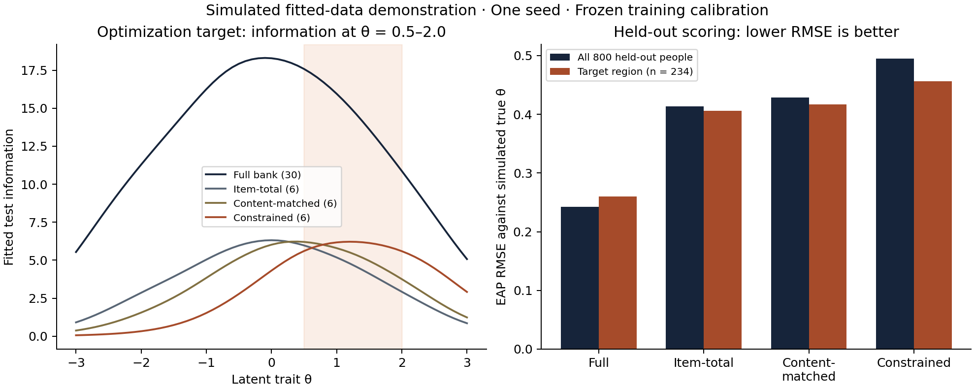
| Form | Training α | Minimum target information | Overall RMSE | Target RMSE |
|---|---|---|---|---|
| Full bank (30) | 0.927 | 10.871 | 0.242 | 0.260 |
| Item-total (6) | 0.817 | 2.924 | 0.413 | 0.406 |
| Content-matched (6) | 0.808 | 3.755 | 0.428 | 0.417 |
| Constrained (6) | 0.774 | 5.595 | 0.495 | 0.456 |
The information objective improves; held-out scoring does not. The constrained form selects items 8, 10, 17, 20, 29, 30. Its minimum target information is 5.595, versus 2.924 for item-total selection. Yet target-region EAP RMSE is 0.456 versus 0.406. The paired RMSE difference is 0.050 (95% percentile bootstrap interval 0.003 to 0.097; 2,000 resamples of held-out people). This interval excludes calibration and selection uncertainty.
Information optimization is conditional on a model and objective. It does not guarantee lower finite-sample EAP error or better decisions. Prior shrinkage, scoring bias and threshold placement are possible contributors; this single experiment does not isolate why the ranking differs. The candidate should therefore be evaluated against the intended scoring and decision criteria before use.
Model checks and boundaries
The training fit converged. The C₂ test is 453.99 on 405 degrees of freedom (p = 0.0465); RMSEA is 0.0087 and SRMSR is 0.0181. The p-value is below .05 despite small approximate-fit indices; these diagnostics are reported together, not treated as automatic proof of fit. Mean training Q₃ is -0.029; zero pairs exceed the descriptive mean-centered Q₃ threshold of .20. Thus this run does not demonstrate an active enemy-pair exclusion. No DIF or readability assessment is claimed.
This initial result uses one seed from a correctly specified generating family and excludes parameter uncertainty and real-world validation. Section 7.2 below repeats sampling, calibration and selection for the same bank. Classification metrics in the downloads use the arbitrary cutoff θ ≥ 1 against simulated true θ. They are not diagnostic sensitivity or specificity for a clinical condition. Fitted information, EAP RMSE and posterior SD answer different questions.
Reproduce and inspect
Download the complete fitted-demo package (ZIP) · Methods and setup · Results JSON · Independent numerical checks · Held-out scores CSV
Extract the ZIP and run from its root. Install R packages mirt, lpSolve and jsonlite, plus Python packages NumPy, SciPy and Matplotlib; the README gives commands and recorded versions.
Rscript scripts/fitted-short-form-demo/run_demo.R
python scripts/fitted-short-form-demo/check_and_publish.py
Python independently checks information and EAP scoring from the frozen R calibration to an absolute error below 10⁻⁹ and selects the same constrained items with SciPy. It does not independently calibrate the GRM. See the mirt calibration documentation and scoring documentation.
7.1 Why the scoring rule matters: bias and variance
To go beyond one holdout sample, we enumerated all 15,625 possible response patterns for each frozen six-item form. Response probabilities use the known generating parameters; scores use the fitted parameters. At each θ, this gives the conditional expected score, bias, variance and mean squared error by direct summation. MSE = bias² + variance. The calculation is conditional on this one fitted bank and its selected forms, rather than a repeated-calibration simulation.
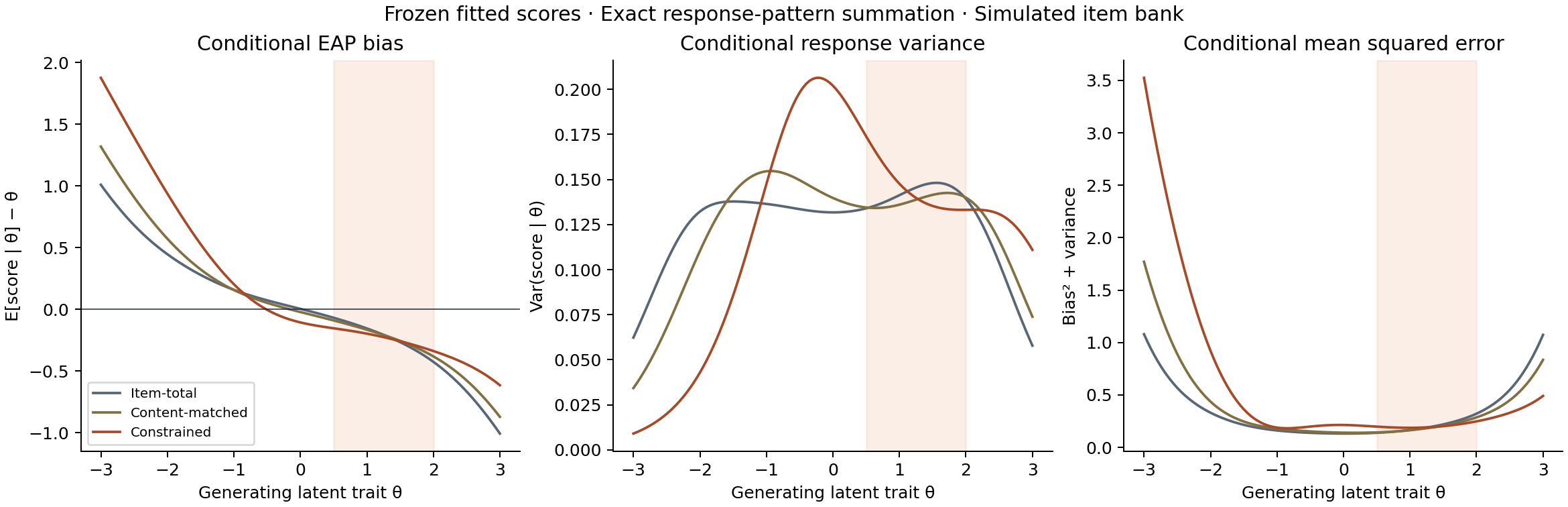
| Six-item form | EAP bias² | EAP variance | Normal-prior RMSE | Flat-grid-prior RMSE |
|---|---|---|---|---|
| Item-total (6) | 0.0371 | 0.1410 | 0.422 | 0.621 |
| Content-matched (6) | 0.0368 | 0.1370 | 0.417 | 0.524 |
| Constrained (6) | 0.0453 | 0.1502 | 0.442 | 0.498 |
Both components contribute in this fitted bank. Under normal-prior EAP, the constrained form has higher integrated squared bias (0.0453 versus 0.0371) and variance (0.1502 versus 0.1410) than item-total selection. Its target mean bias is −0.208 versus −0.173. The population-weighted conditional RMSE is 0.442 versus 0.422; these are model-based expectations over responses and θ, not the finite holdout values of 0.456 and 0.406.
Prior sensitivity changes the ranking, without improving this form’s scoring error. Keeping the same fitted coefficients, item selections, response patterns and scoring grid, replacing the N(0,1) prior with equal grid weights on [−6,6] reduces constrained-form squared bias to 0.0055 but raises variance to 0.2421. Its RMSE increases from 0.442 to 0.498. With this flat-grid posterior mean it performs better than the two comparators, whose RMSEs also worsen. Thus prior weighting affects the comparison, but removing normal-prior shrinkage is not a demonstrated solution. The flat-grid score is a diagnostic perturbation, not maximum-likelihood scoring or an endorsed replacement.
The downloads also include empirical held-out errors in half-unit θ bins, with bin counts. Their error variance includes within-bin variation in θ and bias, so it must not be read as conditional score variance at a fixed θ. This analysis explains the frozen-bank comparison; the repeated-response study below examines stability across calibration samples, while Section 7.3 examines a heuristic selection objective aligned with scoring loss.
Conditional decomposition CSV · Held-out error bins CSV · Prior-sensitivity results JSON
7.2 Repeating calibration and selection across response samples
We fixed the generating bank from the original example and specified seeds 20261101–20261130 before running this extension. Each seed generates a fresh sample of 1,600 training and 800 held-out respondents, recalibrates the GRM, repeats training-only screening and item selection, then scores the held-out respondents with the fitted bank and the same N(0,1) EAP prior. These are 30 response-sample replications under one bank, not 30 different instruments.
30 of 30 attempts completed successfully; 0 failed. Every attempt is retained in the JSON log, including warnings and failure messages. Numerical summaries below use successful attempts. The selection objective, target grid, content requirements, scoring prior and evaluation definitions were unchanged.
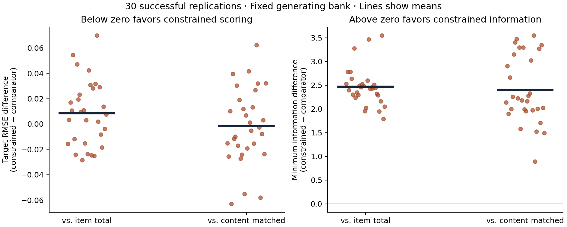
| Comparison | Mean target RMSE difference | 95% Monte Carlo t interval | Constrained target-RMSE wins | Mean minimum-information gain |
|---|---|---|---|---|
| Constrained vs. Item-total | 0.0085 | -0.0011 to 0.0182 | 11/30 | 2.467 |
| Constrained vs. Content-matched | -0.0017 | -0.0129 to 0.0095 | 16/30 | 2.400 |
Mean target-region RMSE was 0.260 for the 30-item bank, 0.423 for item-total selection, 0.434 for content-matched selection, and 0.432 for constrained assembly. The constrained form had lower target-region RMSE than item-total selection in 11 of 30 successful replications. The full bank is a length reference, not a burden-matched comparator.
The constrained form increased minimum target information relative to item-total selection in 30 of 30 successful runs. Both target-RMSE mean-difference intervals include zero in this run; they do not establish equivalence or a consistent average scoring advantage. Across the full population, constrained EAP RMSE was worse than item-total selection in every successful run (mean paired difference 0.074), showing why performance outside the target region also needs evaluation.
This study reports the distribution rather than selecting a favorable seed. Thirty attempts are an illustrative extension, not a precision-powered simulation study; the downloadable summary includes Monte Carlo standard errors and Wilson intervals for win fractions. The generating bank, population and model family remain fixed. These results do not establish clinical performance, generalize across item banks or generalize to all scoring-loss objectives; Section 7.3 tests one such heuristic. Parameter estimation varies across replications, but the original conditional analysis remains tied to its one frozen calibration.
Per-seed metrics CSV · Summary JSON · All attempts, warnings and selected items
# After reproducing the original fitted bank:
Rscript scripts/fitted-short-form-demo/repeat_demo.R
python scripts/fitted-short-form-demo/check_and_publish.py
7.3 Selecting for expected scoring error
We next changed the selection objective while keeping the generating bank, six-item length, two-items-per-domain blueprint, training-only enemy-pair screening, θ = 0.5–2 target region and N(0,1) EAP scoring prior fixed. Seeds 20261201–20261230 supply fresh training and held-out responses, with 1,600/800 people per attempt. They were chosen before this comparison and are separate from the earlier replication seeds.
The new criterion is expected EAP squared error, averaged over a target-truncated normal trait distribution under the fitted training model. It uses no generating item parameters, held-out responses or held-out true θ for selection. Held-out outcomes are read only after the selected candidate is saved.
This is a bounded heuristic search, not a globally optimal solution. Common random numbers generate 1,024 fitted-model design cases. Starting from maximin information and a feasible content-matched form, the search makes up to three best within-domain swaps per start. The five best approximate candidates plus feasible starts are evaluated by summing all 15,625 response patterns, with a 0.05 trapezoidal target-θ grid and the same 61-point EAP scoring grid. Exact response-pattern summation is not exact θ integration. Including maximin among finalists guarantees no worse fitted-model loss than that candidate, without guaranteeing better held-out error or global optimality.
30 of 30 comparisons completed successfully; 0 failed. Failure records are retained. Selection effort differs from MILP assembly and this is not a comparison of solver speed.
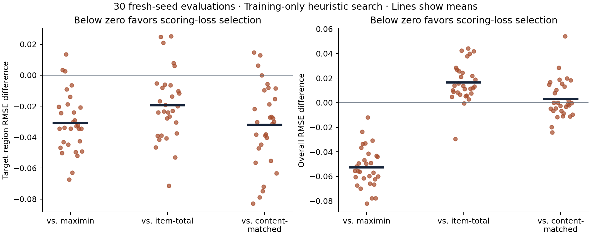
| Comparison | Mean paired difference | 95% Monte Carlo t interval | Scoring-loss wins |
|---|---|---|---|
| Scoring-loss vs. Maximin information | -0.0308 | -0.0380 to -0.0236 | 27/30 |
| Scoring-loss vs. Item-total | -0.0194 | -0.0278 to -0.0109 | 25/30 |
| Scoring-loss vs. Content-matched | -0.0320 | -0.0419 to -0.0220 | 26/30 |
Mean target-region RMSE was 0.402 for scoring-loss selection, 0.433 for maximin information, 0.421 for item-total selection and 0.434 for content-matched selection. The paired mean target-RMSE interval favors scoring-loss selection in this fixed-bank experiment. Fitted-model target MSE decreased by 0.0243 on average relative to maximin; this model-based objective change is distinct from the held-out RMSE comparison.
The gain is specific to the target and scorer. Relative to maximin, scoring-loss selection changed minimum target information by -0.649 on average. Relative to item-total selection, its overall-population RMSE difference was +0.016 on average (positive is worse). Lower target-region scoring error therefore does not mean better performance for every trait level or every study purpose.
These results address alignment between one scoring rule and selection objective. The change includes both the error criterion and aggregation (worst-case information versus target-weighted mean squared error), as well as the search procedure; it does not isolate the contribution of each component. They do not identify a universally best short form. Search is heuristic, the target integral is numerical, calibration uncertainty is not modeled in selection, and only one generating item bank is used. No clinical validity, DIF, readability or external-population claim is added. The next generality check would vary generating banks and trait distributions.
Scoring-loss summary JSON · Per-seed metrics CSV · All selection/evaluation attempts · Updated complete reproducibility package
# After generating the original bank:
Rscript scripts/fitted-short-form-demo/prepare_scoring_loss.R
python scripts/fitted-short-form-demo/evaluate_scoring_loss.py
python scripts/fitted-short-form-demo/check_and_publish.py
7.4 Sensitivity to the heuristic search settings
We chose ten evenly spaced frozen calibrations (seeds 20261201, 20261204, …, 20261228) from the fresh-seed study before this check. No held-out outcomes were used to choose settings or evaluate this sensitivity analysis. The inputs are fitted training parameters, training-derived item subsets and enemy-pair metadata. These are ten calibrations from one generating bank, not ten different generating banks.
The nine settings include the published default; 256 and 4,096 design cases; one and six swap rounds; either original search start alone; another design draw; and two extra feasible random starts. Design sample sizes are nested around the original 1,024-case draw. Apart from the factor changed, settings retain the default 1,024 cases, three rounds and two starts. Every setting keeps the maximin and feasible content-matched anchors among finalists. Extra random starts are also finalists. Thus the start check concerns search paths, with shared anchor safeguards, rather than removing all influence of those anchor forms.
90 of 90 search attempts completed successfully; 0 failed. Paired summaries use 10 calibrations for which every setting completed. All default replays matched the published items and fitted-model loss. Failure details, if any, remain in the attempt log.
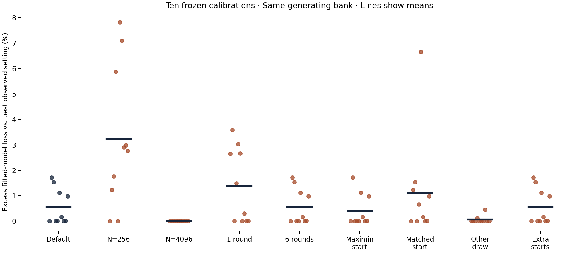
| Setting | Identical items | Mean shared items | Mean excess loss | Worst excess loss |
|---|---|---|---|---|
| Published default | 10/10 | 6.0/6 | 0.55% | 1.72% |
| 256 design cases | 2/10 | 4.8/6 | 3.24% | 7.81% |
| 4,096 design cases | 4/10 | 5.4/6 | 0.00% | 0.00% |
| 1 swap round | 0/10 | 4.9/6 | 1.37% | 3.58% |
| 6 swap rounds | 10/10 | 6.0/6 | 0.55% | 1.72% |
| Maximin search start | 9/10 | 5.9/6 | 0.40% | 1.72% |
| Content-matched search start | 7/10 | 5.6/6 | 1.13% | 6.65% |
| Alternate design draw | 2/10 | 5.2/6 | 0.06% | 0.45% |
| Two extra search starts | 10/10 | 6.0/6 | 0.55% | 1.72% |
The published default’s fitted-model loss exceeded the best observed setting by 0.55% on average, with a worst-calibration gap of 1.72%. Changing an item set does not by itself imply a large scoring difference; conversely, similar average losses can hide an important individual calibration gap.
Six rounds and two extra starts each recovered the default item set in 10/10 and 10/10 calibrations, respectively. The 4,096-case design matched default items in 4/10 and attained the best observed loss in every calibration in this run. The 256-case design’s largest excess loss was 7.81%. These patterns indicate greater sensitivity to the simulation design than to the tested increases in rounds or starts; they do not establish that a larger design improves held-out performance.
This is a bounded sensitivity check. The best-observed reference is selected from the same tested settings and is descriptive, not an unbiased estimate of global regret. We neither promote the best setting using held-out outcomes nor replace the published default or its earlier performance claims. The check varies one factor at a time, omits interactions and examines one alternative design draw. It does not prove search convergence or robustness across generating banks, populations or instruments.
Stability summary JSON · Per-calibration settings CSV · All attempts and configurations
# Uses the existing fitted training banks; no recalibration is required:
python scripts/fitted-short-form-demo/search_stability.py
python scripts/fitted-short-form-demo/check_and_publish.py
References
- Christensen, K. B., Makransky, G., & Horton, M. (2017). Critical values for Yen’s Q₃: Identification of local dependence in the Rasch model using residual correlations. Applied Psychological Measurement, 41(3), 178–194.
- Chalmers, R. P. (2012). mirt: A multidimensional item response theory package for the R environment. Journal of Statistical Software, 48(6), 1–29.
- Lord, F. M., & Wingersky, M. S. (1984). Comparison of IRT true-score and equipercentile observed-score "equatings." Applied Psychological Measurement, 8(4), 453–461.
- Samejima, F. (1969). Estimation of latent ability using a response pattern of graded scores. Psychometrika Monograph Supplement, 34(4, Pt. 2), 100.
- van der Linden, W. J. (2005). Linear models for optimal test design. Springer.
- Yen, W. M. (1984). Effects of local item dependence on the fit and equating performance of the three-parameter logistic model. Applied Psychological Measurement, 8(2), 125–145.
Further work
The following extensions could test the limits of these findings. They have not been completed in this demonstration.
- Different item banks: vary threshold coverage and discrimination to test whether the findings extend beyond the current bank.
- Population and calibration conditions: vary trait distributions and calibration sample sizes, and account for item-parameter uncertainty.
- Model departures: examine multidimensionality, local dependence and missing responses.
- Broader search checks: test interactions among search settings, additional random draws and wider candidate searches.
- Other decision goals: compare target-region scoring error, overall accuracy and classification losses under explicit study priorities.
- Real-data validation: use appropriately permitted instruments and independent data to assess content coverage, subgroup performance and score comparability.